Electrostatic Potential
The static electric field is a conservative field, that is, \(\exists V: -\vec{\nabla} V = \vec{E}\), or similarly, \(\oint_c \vec{E} \cdot d\vec{s} = 0\).
We consider the electric field to be negative the gradient of \(V\), because we imagine a positive charge “flowing down hill,” i.e., going from higher to lower potential.
Defining the potential in terms of the electric field:
\[ \int_c \vec{\nabla} V \cdot d\vec{l} = - \int_C \vec{E} \cdot d\vec{l} \]
Applying FTC and the chain rule:
\[ \int_{t_i}^{t_f} \vec{\nabla} V(\vec{l}(t)) \cdot \vec{l'}(t) dt = RHS\]
\[ \int_{t_i}^{t_f} \frac{d}{dt} \left ( V(\vec{l}(t)) \right ) dt = V(\vec{l}(t_f)) - V(\vec{l}(t_i)) = RHS\]
Define: \(\vec{l}(t_f) = B\) and \(\vec{l}(t_i) = A\)
\[ V(B)-V(A) = - \int_A^B \vec{E} \cdot d\vec{l} \]
The important thing to notice here is that we are actually defining the change in potential, \(\Delta V\), between two points, \(A\), and \(B\). Instead, it is useful to fix one of these points. We define the potential function \(V(x)\) w.r.t the constant reference potential \(V_0\), where \(V_0 = V(x_0)\). What has physical meaning is the differential, so the constant chosen for \(V_0\) doesn't matter.
\[ V(x) - V(x_0) = - \int_{x_0}^{x} \vec{E} \cdot d\vec{l} \]
\[ V(x) = V_0 - \int_{x_0}^{x} \vec{E} \cdot d\vec{l}\]
In practice, for a point charge we almost always choose 𝑉(∞)=0. More generally, if there is some convenient “reference at infinity” or “reference at the conductor’s surface,” one uses that.
Electric potential for a point charge (Coulomb potential)
\[ \vec{E} = \frac{1}{4\pi \epsilon_0} \frac{q}{r^2} \hat{r}\]
\[ V(r_f) - V(r_i) = \frac{-q}{4\pi \epsilon_0} \int_{r_i}^{r_f} \frac{1}{r^2} dr = \frac{q}{4\pi \epsilon_0} \int_{r_f}^{r_i} \frac{1}{r^2} dr = \frac{q}{4 \pi \epsilon_0} \left(-\frac{1}{r} \right)^{r_i}_{r_f}\]
\[ V(r_f) - V(r_i) = \frac{q}{4 \pi \epsilon_0} \left( \frac{-1}{r_i} - \frac{-1}{r_f} \right) = \frac{q}{4 \pi \epsilon_0} \left( \frac{1}{r_f} - \frac{1}{r_i} \right)\]
Now we can consider the reference point at infinity, choose \(V(r_i) = V_0 = 0\) and let \(r_f = r\). As the reference point goes to infinity \(r_i\) approaches infinity.
\[ V(r) = \frac{q}{4 \pi \epsilon_0} \lim_{r_i \to \infty} \left( \frac{1}{r} - \frac{1}{r_i} \right) = \frac{q}{4 \pi \epsilon_0} \frac{1}{r}\]
Superposition of voltages
For any point, \(P\), we can determine the total voltage at that point, by taking a linear combination of the voltages produced by each individual charge. The important thing to note however, is that each voltage must be w.r.t the same reference.
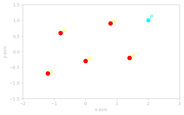
For this charge distribution we can consider the function \(V(r)\) to have its reference at infinity. Then the total voltage at P can be expressed in the form:
\[ V_P = k_e \sum \frac{q_i}{r_i}\]
This property allows us to extend our toolbox towards continuous charge distributions by turning the discrete sum into a continuous integral.
\[ V_P = k_e \int \frac{dq}{r}\]
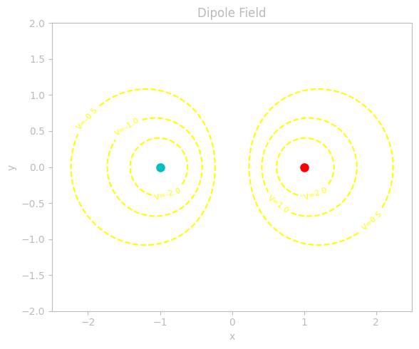
Equipotential Surfaces
Any surface (in three dimensions) or curve (in two dimensions) for which the electric potential 𝑉 remains constant is called an equipotential surface. Because \(\Delta V = 0\) along this surface, no net work is required to move a charge anywhere on the surface; the electric force does no work if you remain on that same potential value.
Another key property is that equipotential surfaces always intersect electric field lines at right angles (orthogonally). Intuitively, you can think of each equipotential “shell” as a level set of the potential function 𝑉. From vector calculus, \(\vec{E} = - \vec{\nabla}V\), and the gradient \(\vec{\nabla} V\) always points in the direction of steepest increase of 𝑉. Since a level set is, by definition, everywhere constant in value, the gradient must be perpendicular to it. This geometric fact leads directly to the perpendicular crossing of field lines.
Potential energy vs. Electric potential
- The work done in taking a charge around a closed loop in a static electric field generated by fixed charges is zero.
- The work done by moving charges through a static electric field is path independent.
- The electrostatic force is a conservative force thus, we can define the work by the force as: \(W = U_1 - U_2 = -\Delta U\).
- The electrostatic potential (V) is the potential energy function per unit charge: \(\Delta V = \frac{\Delta U}{q}\)
- Potential measured in units of Volts, energy is measured in units of electronVolts.